Electric Potential Energy and Work

The two pictures above show the arrangement needed to ensure the brightest light from the bulbs. The bulbs each are connected to one end of the battery arrangement, and the other end of the respective bulb holders are touching with 1 cable running to the other end of the battery. In this arrangement the bulbs are getting the required energy at the same time rather than one getting more than another, which would happen in a linear arrangement where one bulb gets most of the energy first.

This arrangement shows the least brightest light. The battery are placed parallel to each other and one bulb receives the little bit of energy before the other bulb, resulting in one bulb being barely lit and the other not being lit at all.

The picture above is our illustration of the bulb and battery arrangements shown above. The top pictures are Mario's artistic representations while the bottom two pictures are more scientific representations of the bulbs and batteries. The batteries are represented by 2 parallel lines, the shorter being negative and the larger being positive and the bulbs are represented by swirls.

This is an experiment Professor Mason did in class in which he heated up water with a cup of noodles heater (water heater) that was hooked up to a voltage regulator.

This is the graph of temperature vs. time of the experiment mentioned above.

He doubled the voltage and repeated the experiment. As seen doubling the voltage more than doubled the temperature meaning that there are some other factors involved which accounted for the sharp rise in slope.

The picture above shows our attempt at figuring out why the slow in the above experiment jumped 7 times higher. We determined that the change in resistance was so negligible that we could consider it constant. So because of that we could determine that doubling the voltage would double the current, meaning that the power supplied would quadruple. In class we showed a near 7 time jump in slope, so there was probably a mistake in the experiment since the change should've been closer to 4 times larger.

In the above two pictures we calculated the amount of work needed to get the cart from point to point C. We determined that any path taken would result in the same amount of work.

We also symbolically showed the work needed to get from one point to another in an electric field. With distance D, A had the least amount of work since it was parallel to the field, B had the most since it was perpendicular to the field and C was in between since it had an angle less than 90 degrees to the field.

The picture on the right shows that a circle would have equal potential lines when a is going out at all possible angles from a central location. On the left we derive the formula for a change in voltage from an infinitely large distance (which would end up being zero) to a set distance r.

The picture above illustrates what we though the code provided by Professor Mason would produce.

The picture above shows my arrangement of charges (blue, red, yellow) and 3 locations (green spheres) where we observed what the electric potential would be. This was achieved by multiplying each charge by 1/4*pi*epsilon not and dividing that by the distance between the observation location and the actual charge. The three were then added together to find the total electric potential at each location.

This work shows that the net electric potential was zero for 2 equal but opposite charges.

The picture above shows what we though the difference between plagiarism and collaboration was. Professor Mason brought this up while talking about labs to ensure we knew what not to do when creating our blogs.

Current and Resistance

In the picture above we light the bulb by ensuring that the cable is touching one end of the battery and the side of the bulb and that the bulb's bottom is touching the other end of the battery. We could have also lit the bulb by touching the cable to the bottom of the bulb and placing the side of the bulb on the battery. This works because the charge goes from the battery into the bulb and then flows out back into the battery. This keeps the flow of energy going.

We show the same thing we did above but with 2 batteries.

This is an electroscope. You touch the top bulb with an object and the two plates inside the box will move if the object has a charge.

In the video above Professor Mason shows us how the electroscope works. He introduces a charge to the rod by rubbing it with animal fur, then touches the electroscope and we see the plates move, confirming that the rod has a charge.

The picture above illustrated 2 methods where the bulb could be lit by a battery and 2 methods where the bulb would not be lit. The right most picture was something we accidentally did at first, without the fire of course. The bottom picture shows how to make the bulb light with 2 batteries.

We assumed that nothing would happen if we connected the positive end of the battery to the electroscope and we were correct. We also explain why a close circuit connection is required to light the bulb. Electrons flow into the bulb but also flow out, ensuring that it does not get full.

In the above picture we use a 4 amp bulb and battery with an old style multimeter and we illustrate the same thing we did above by creating a close circuit connection in which the bulb could light. We wanted to determine if flow of energy outside of the bulb would match flow of energy to the bulb, so we tested it at both ends, and in both situations the meter read 4 amps, meaning that they were equal, there was no energy lost.

We assumed that the charge of an electron, cross sectional area, drift velocity, and number density were required to find the charge. In the picture above we were able to find drift velocity with some givens.

Professor Mason adds a current to a wire typically found in a toaster. We wanted to see if there was any relationship between current(Amps) and potential energy (volts).

The picture above is the graph of the experiment Professor Mason performed in class. There is a linear relationship between current and potential energy.

Professor Mason also tried the same thing with the light bulb, but unfortunately the bulb kept blowing.

This is what we assumed the graph would look like and we were correct. We also assumed that the opposite relationship would be linear, which was also correct.

We determined that if the diameter of a cable goes up the resistance goes down. Resistance also goes up with length. We also determined that material used also factors into how much resistance there is.

Gauss' Law

The picture above illustrates Gauss' Law. We have 3 charges, 1 negative and 2 positive. We enclosed them separately and together to illustrate the flux going through the surfaces. Gauss' Law is charge enclosed over epsilon not (8.854 * 10^-12).

In this picture we say that q is similar to flux and that flux is equal to the integral of E*cos(theta)*da. We also found the units of our electric constant and our energy field.

The top 4 pictures are of an experiment that Professor Mason did in class. He demonstrated the charge inside and outside of a gated cylinder. A negative charge was sent into the cylinder. My assumption was that nothing would happen to the pieces of foil inside and outside of the cylinder. I was wrong though since I did not realize that the cage was essentially charging those pieces on the outside, and eventually they would be fully charged with a negative charge and would then be repelled by the negatively charged cage. The pieces of foil on the inside were unaffected since the charge of the cage goes outwards.

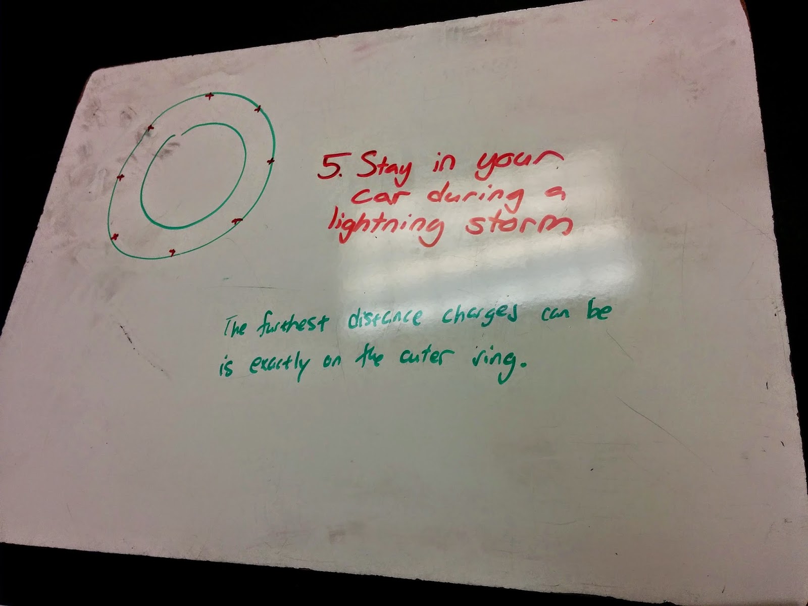
We assumed that if you were in your car during a lightning storm you should stay inside of the car. I assumed this since the charge should go outward and that the tires were acting as insulators, passing the charge to the ground around you, meaning you should definitely not get out.

In the top two pictures we were answering questions regarding the area, circumference, area, and volume of a sphere. We wrote how a change in radius would affect the volume or area. We also noted that the dot product between E and dA is the same as EdA because the vectors are parallel since the electric field vector is normal to the plane.

The two videos above show the effect of the electric field created by the microwave onto the various metal objects placed into it. The steel wool, which I unfortunately do not have a video/picture of, sparked at its ends. The fork had sparks at it's tips. The CD sparked on the shiny side of the disk, since that is the metal part. The filaments inside of the light bulb lit up and heats up the argon gas inside of the bulb which creates the light we see in the video.

We found the electric field for a cylinder with charge density lambda. First we found the surface area, which we did in the top picture. We were able to drop the 2*pi*r^2 since the top and bottom of the cylinder would cancel out, which left us with 2*pi*r*L. We plugged everything in to find the electric field on the bottom right.

In this picture we found the gravity of the earth by using the gravitational form of Gauss' Law.

Flux

Above we see what would happen if an electron went in between two plates, one being positive and one being negative. We see that the electron would slowly go toward the positive plate and go away from the negative plate. On the right we see a dipole with two charges on it, and arrows illustrating an electric field. The dipole would want to straighten out since the field would cause the positive charge to go right and the negative charge to go left.

Here are a few equations we derived for torque. We found that the sum of torque is the cross product between the dipole moment vector and the electric field vector. On the bottom right we have some equations for work.

The above picture illustrates what we thought the program provided by Professor Mason would do ( in red ) and the correct path those vectors should take (in green). There is a positive charge (red small circle) and a negative charge (green small circle).

The picture above is the program Professor Mason provided modified to show how the field should look in 3 dimensions. The original program, prior to adding the Z axis, would draw the orange arrows.

The picture above shows the flow of the electric field between a positive and negative charge. Professor Mason added the blue negative charge to our illustration, and on the bottom right we show what affect that would have. The two negative charges would repulse one another.

First we found the units for flux in the top right corner then we determined the normal vectors for the objects drawn.

In the picture above we calculate flux on a box. In 3 dimensions it was hard to illustrate so we opened the box up. 4 of the sides of the box were parallel with the electric field so flux would be zero. We also see that the two sides affected by the field, colored in green, would cancel each other out, meaning that the total flux of the box would be zero.

Electric Fields

The above picture is a list that describes electric fields.

This picture shows instructions on what to do in VPython in order to recreate that picture with vectors representing the electric field.

The above picture shows my modification to the code provided by Professor Mason. This program illustrates the 3 dimensional electric field (the arrows) created by the positive charge at the center.

The picture of the graph above is what I assumed the code provided by Professor mason would result in. I was incorrect though because I forgot that the number placed in the X component does not point to a location, but in fact is a direction and length. The picture should have shows all arrows pointing to the right.

The above picture shows the calculations for finding the x and y components of an electric field vector using the formula (kq/r^3)x and (kq/r^3)y. The picture of this picture shows the magnitude of the electric field vector.

Here we found the total electric field vector for the point on the y axis. Since the charges are equal and opposite they cancel out making the total electric field vector a 0 vector.

The above picture shows our excel file which has a list of radii, their corresponding energy fields with the given k and q, then the sum of those energy fields on the bottom.

This picture is similar to the one above except that it also shows the electric field in the Y and X axes, and their summations at the bottom. Since the point that we were checking was at the center of a horizontal pole below it, the electric field cancels out.

This picture shows the integral to find the electric field across a line.

3D Computer Modeling

The above picture shows how I completed the challenge from the 3D Objects Video.

Afterward, I commented out two of the arrows with #, then I shortened the length of the remaining arrow by half and flipped it so it would point in the opposite direction. As you can see the arrow is now barely visible on the orange sphere.

Note on the Syntax Errors Video: ALWAYS CAPITALIZE BOB, it may one day save your life and the lives of your loved ones.

Above is my Chipmunk themed solution for the challenge in the Variable Assignment video.

I doubled the distance that Theodore was from the y-axis and since all of the arrows were based on variables, rather than numbers, they adjusted to still be connected. The picture also shows the printed position attribute of Simon. Alvin is usually hogging the spotlight so I figured Simon and Theodore could use this win.